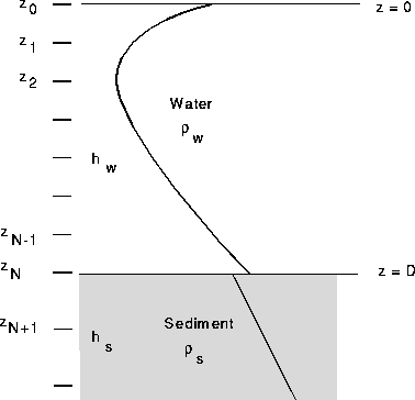
Figure: Finite-difference mesh for an interface.
Frequently ocean acoustic problems involve discontinuities in the sound speed or density, for instance in passing from ocean to sediment. Such problems are treated by dividing the problem into layers such that within a layer these material properties vary smoothly. Within a layer the previous finite difference equations are applicable. At the interface one then derives a special condition to tie together the individual layers.
As an example, we consider a a single interface between two layers
representing the water and the sediment. Within each layer we
construct independent finite-difference meshes with grid spacing
 and
and  as illustrated in Fig. 3.2. In the water, the
finite-difference approximation to Eq. (
as illustrated in Fig. 3.2. In the water, the
finite-difference approximation to Eq. (![]() ) is
) is
and in the sediment the finite-difference approximation is

At the interface, the pressure must be continuous,
a condition which is imposed implicitly by allowing for a unique
value  at the interface. We must also impose
continuity of normal velocity, that is,
at the interface. We must also impose
continuity of normal velocity, that is,

where  and
and  denote the densities in the water and
sediment respectively. This interface condition can then be
approximated by,
denote the densities in the water and
sediment respectively. This interface condition can then be
approximated by,
where we have used the backward difference formula for the water and
the forward difference for the sediment. Furthermore,
 denotes the limiting value of the sound
speed at the interface as approached from z<D (
denotes the limiting value of the sound
speed at the interface as approached from z<D ( ) and z>D
(
) and z>D
( ).
Rearranging we obtain,
).
Rearranging we obtain,
Note that if  ,
,  and
and  is continuous we
obtain the same finite-difference formula given in Eq. (
is continuous we
obtain the same finite-difference formula given in Eq. (![]() )
for a point not on an interface.
)
for a point not on an interface.
This process can obviously be repeated for every interface in the problem and, just as for the single layer case, leads to a symmetric matrix eigenvalue problem. Incidentally, the resulting problem is precisely equivalent to what one would obtain by using finite elements with hat-shaped basis functions and `mass-lumping'.
