The Munk profile[47] is an idealized sound speed profile; however, it allows us to illustrate many features that are typical of deep-water SSP's. In its general form, the profile is given by

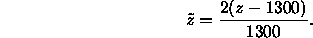
The quantity  is taken to be

while the scaled depth  is given by
The resulting profile is plotted
in Fig. 2.10. The bottom is taken to lie at a depth of
 . In addition, the bottom sound speed is
  and the
bottom density is
and the
bottom density is  . Taking a source frequency of
  , we
then obtain the modes shown in Fig. 2.11. (An analytic solution for the
modes is not available in this case so we use a numerical technique
as described in Chap. 3.) Notice that the mode shapes are no longer
perfect sinusoids, however the mth mode still has m zero
crossings. In addition, the modes are oscillatory near the sound
channel axis and exponentially decaying in a layer near the surface
and near the bottom. The size of the oscillatory region is larger
for the higher order modes.
, we
then obtain the modes shown in Fig. 2.11. (An analytic solution for the
modes is not available in this case so we use a numerical technique
as described in Chap. 3.) Notice that the mode shapes are no longer
perfect sinusoids, however the mth mode still has m zero
crossings. In addition, the modes are oscillatory near the sound
channel axis and exponentially decaying in a layer near the surface
and near the bottom. The size of the oscillatory region is larger
for the higher order modes.
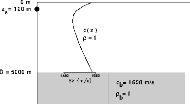
Figure: Schematic of the deep-water problem.
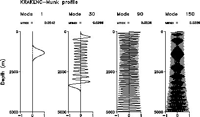
Figure: Selected modes for the deep-water problem.
Some insight into the behavior of the modes can be obtained from the WKB approximation[48]. The WKB approximation to the eigenfunctions is given by
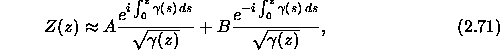
where
Thus, locally the solution assumes the oscillating form of sines and
cosines near the sound channel axis (where  is real) and
transitions to a solution involving exponentially growing and
decaying functions near the surface and bottom (where
is real) and
transitions to a solution involving exponentially growing and
decaying functions near the surface and bottom (where  is
imaginary). The depths where this transition occurs are the
turning points and are precisely defined by depths where
is
imaginary). The depths where this transition occurs are the
turning points and are precisely defined by depths where
 . In addition, the amplitude term is seen to be
governed by
. In addition, the amplitude term is seen to be
governed by  so that as we move away from the sound
channel axis (where
so that as we move away from the sound
channel axis (where  is large) towards the turning point
(where
is large) towards the turning point
(where  is small) the amplitude tends to increase. At the
turning point the WKB approximation is actually singular. The correct
solution, however, has a smooth behavior in the transition layer as
may be seen in Fig. 2.11.
is small) the amplitude tends to increase. At the
turning point the WKB approximation is actually singular. The correct
solution, however, has a smooth behavior in the transition layer as
may be seen in Fig. 2.11.
In Fig. 2.12 we illustrate the effect of using different numbers of
modes to calculate transmission loss. The source depth is chosen to
be  . Figure 2.12(a) includes only the waterborne
modes, that is modes which have their lowest turning point above the
ocean bottom. These modes (modes 1 to 63) are exponentially decaying
below this turning point and in this sense are not bottom
interacting. In ray terms these modes correspond to paths which are
refracted away from the bottom.
. Figure 2.12(a) includes only the waterborne
modes, that is modes which have their lowest turning point above the
ocean bottom. These modes (modes 1 to 63) are exponentially decaying
below this turning point and in this sense are not bottom
interacting. In ray terms these modes correspond to paths which are
refracted away from the bottom.
The transmission loss shows a convergence zone type of pattern involving a beam of energy that emerges from the source and refracts under the influence of the ocean sound speed profile. Since we are using a restricted number of modes, we in effect are producing an angle-limited source. We observe that the transmission loss shows large shadow zones where the acoustic field is negligible. These quiet zones result not from the depth-dependence of the eigenfunctions but from the phasing in range which causes the modes to add up destructively.
In Fig. 2.12(b) we have added in the bottom bounce modes (modes 64 to 102). These modes have no turning point and correspond to ray paths which strike the bottom at a subcritical angle. Including these modes effectively widens the source beam-width. A second beam is now visible emanating from the source and reflecting off the bottom.
In Fig. 2.12(c) we have added in a large number of leaky modes
(modes 103 to 400). As discussed earlier these modes are leaky in
the sense that they are displaced from the real axis and therefore
lose energy as a function of range. In ray terms, they corresponds
to paths which strike the bottom above the critical angle and
therefore are very weakly reflected. In the transmission loss plot
we can see that the source angle has now been opened up to  revealing the full Lloyd mirror pattern of beams. (The Lloyd mirror
results from constructive and destructive interference between the
source and its image reflected in the ocean surface.)
revealing the full Lloyd mirror pattern of beams. (The Lloyd mirror
results from constructive and destructive interference between the
source and its image reflected in the ocean surface.)

Figure: Transmission loss for the deep-water problem including (a)
waterborne modes only, (b) bottom bounce modes and (c) leaky modes.