SCHOLTE

  
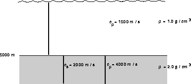
Figure: Schematic of the SCHOLTE problem.

This problem is a version of the Pekeris waveguide but with an elastic half-space as the bottom. This type of problem has a Scholte mode with a phase velocity less than the slowest speed in the problem. (Since the source and receiver are many wavelenghts from the interface the Scholte mode is not actually important for the transmission loss calculation.)

'Scholte waveguide'
10.0
1
'NVM'
500 0.0 5000.0
   0.0 1500.0 /
5000.0 1500.0 /
'A' 0.0
5000.0 4000.0 2000.0 2.0 /
1400.0 2000.0
1000.0                    ! RMAX (km)
1  500.0 /                ! NSD  SD(1:NSD)
1 2500.0 /                ! NRD  RD(1:NRD)

 KRAKEN- Scholte waveguide
 Frequency =   10.00     NMEDIA =   1


     N2-LINEAR approximation to SSP
     Attenuation units: dB/m
     VACUUM


      Z          ALPHAR     BETAR      RHO       ALPHAI     BETAI


          ( Number of pts =   500  RMS roughness =  0.000E+00 )
      0.00      1500.00      0.00     1.00       0.0000    0.0000
   5000.00      1500.00      0.00     1.00       0.0000    0.0000

                                 ( RMS roughness =  0.000E+00 )
     ACOUSTO-ELASTIC half-space
   5000.00      4000.00   2000.00     2.00       0.0000    0.0000

 CLOW =   1400.0      CHIGH =   2000.0    
 RMAX =    1000.000000000000    

 Number of sources   =            1
   500.0000    

 Number of receivers =            1
   2500.000    

 Mesh multiplier   CPU seconds
        1             5.61    
        2             6.51    
        4             4.64    

    I           K                ALPHA         PHASE SPEED
    1   0.4400982929E-01   0.0000000000E+00    1427.677728    
    2   0.4188306870E-01   0.0000000000E+00    1500.173101    
    3   0.4186856672E-01   0.0000000000E+00    1500.692715    
    4   0.4184439022E-01   0.0000000000E+00    1501.559773    
    5   0.4181052921E-01   0.0000000000E+00    1502.775838    
    6   0.4176696933E-01   0.0000000000E+00    1504.343123    
    7   0.4171369148E-01   0.0000000000E+00    1506.264510    
    8   0.4165067147E-01   0.0000000000E+00    1508.543581    
    9   0.4157787955E-01   0.0000000000E+00    1511.184643    
   10   0.4149527997E-01   0.0000000000E+00    1514.192774    
   11   0.4140283053E-01   0.0000000000E+00    1517.573853    
   12   0.4130048217E-01   0.0000000000E+00    1521.334613    
   13   0.4118817854E-01   0.0000000000E+00    1525.482682    
   14   0.4106585562E-01   0.0000000000E+00    1530.026639    
   15   0.4093344142E-01   0.0000000000E+00    1534.976071    
   16   0.4079085559E-01   0.0000000000E+00    1540.341632    
   17   0.4063800914E-01   0.0000000000E+00    1546.135118    
   18   0.4047480418E-01   0.0000000000E+00    1552.369538    
   19   0.4030113364E-01   0.0000000000E+00    1559.059197    
   20   0.4011688100E-01   0.0000000000E+00    1566.219793    
   21   0.3992192010E-01   0.0000000000E+00    1573.868514    
   22   0.3971611492E-01   0.0000000000E+00    1582.024153    
   23   0.3949931943E-01   0.0000000000E+00    1590.707232    
   24   0.3927137754E-01   0.0000000000E+00    1599.940135    
   25   0.3903212305E-01   0.0000000000E+00    1609.747258    
   26   0.3878137986E-01   0.0000000000E+00    1620.155170    
   27   0.3851896232E-01   0.0000000000E+00    1631.192776    
   28   0.3824467597E-01   0.0000000000E+00    1642.891500    
   29   0.3795831866E-01   0.0000000000E+00    1655.285463    
   30   0.3765968244E-01   0.0000000000E+00    1668.411654    
   31   0.3734855636E-01   0.0000000000E+00    1682.310086    
   32   0.3702473075E-01   0.0000000000E+00    1697.023903    
   33   0.3668800348E-01   0.0000000000E+00    1712.599409    
   34   0.3633818906E-01   0.0000000000E+00    1729.085975    
   35   0.3597513167E-01   0.0000000000E+00    1746.535736    
   36   0.3559872314E-01   0.0000000000E+00    1765.002998    
   37   0.3520892659E-01   0.0000000000E+00    1784.543272    
   38   0.3480580404E-01   0.0000000000E+00    1805.211941    
   39   0.3438954040E-01   0.0000000000E+00    1827.062890    
   40   0.3396044231E-01   0.0000000000E+00    1850.148255    
   41   0.3351886824E-01   0.0000000000E+00    1874.521915    
   42   0.3306503451E-01   0.0000000000E+00    1900.250643    
   43   0.3259872074E-01   0.0000000000E+00    1927.433091    
   44   0.3211925126E-01   0.0000000000E+00    1956.205410    
   45   0.3162787575E-01   0.0000000000E+00    1986.597316

  
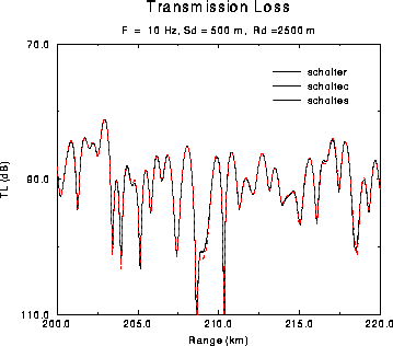
Figure: Transmission loss for the SCHOLTE problem.